Volatility, What a Drag

Over the past couple of months, investors of all types have likely been caught off guard by global events that caused massive swings in the market value of their portfolio holdings. Unfortunately, some have realized that their investments are far too risky and have lost more than they could tolerate. The old gambler’s adage of not risking more than you are willing to lose holds true for investors as well – but how do we know how much is really at risk?

In this first post of a multi-part blog series about understanding risk, I will begin by exploring volatility, a common measure of risk relating to uncertainty. I’ll use explanations and examples, which will lead to a simple framework for investors to understand their own risk tolerance in the context of volatility.

What is Volatility?

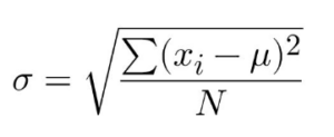
Volatility is a proxy for uncertainty in returns on an investment. In finance, it is most often quantified as the standard deviation of returns on an asset or portfolio of assets. In simple terms, standard deviation tells us how variable returns are when compared to their average return. The higher the standard deviation, the larger the probable range of return values. For those interested, the formula is as follows:

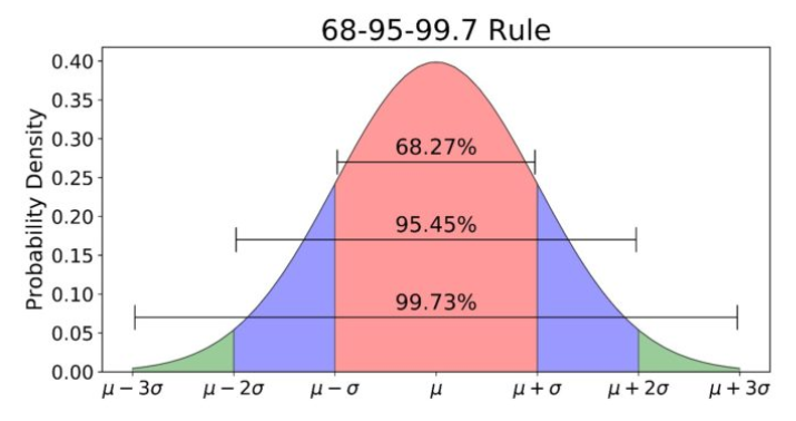
I must mention that the calculation of standard deviation assumes that the data follows a normal distribution. One small but important caveat is that in practice, financial data doesn’t follow a normal distribution and often exhibits a high degree of skewness or kurtosis resulting in “fat tails.” However, these concepts are out of the scope of this blog post and I will aim to explore this nuance in future posts. For now, we can say that financial datasets come close enough to normally distributed for standard deviation to be used as a good approximation of variability. (Click here if you’d like more information on the normal distribution.)

To put the concept of standard deviation into context, it’s best to look at an example. Consider a series of annual returns on a risky asset, which gives us an average return of 5% and a standard deviation of 5%. What this tells us is that in any given year, there is a 68% chance that the return on the asset will be between 0% and 10% (1 standard deviation on either side of the average). Furthermore, there is a 95% chance that the return will fall between -5% and 15% (2 standard deviations) and a 99.7% chance that the return will fall within -10% and 20% (3 standard deviations). This helps us understand the probable range of returns we can expect from an investment. See the below illustration:

How Does Volatility Impact Returns?

Naturally, as we increase volatility, we increase the range of probable outcomes. If we double the volatility in our previous example and hold the average return the same, we end up with 95% confidence that a given year’s return will lie somewhere between -15% to 25%. Some people may look at this and say that they would be willing to accept the greater probability of negative outcomes for the seemingly equivalently greater probability of higher positive outcomes. While it is true for this example that in any given year the increase in probability of below average returns is exactly offset by an increase in above average returns, this doesn’t tell the whole story about the impact on an investment portfolio over time.

Financial returns data is an example of time series data that is geometrically linked rather than arithmetically linked. This means that returns are multiplied together and are path dependent, rather than just simply being added together and independent of the order in which they occur. As a result, negative returns have an asymmetric impact on wealth when compared to positive returns. To illustrate this effect, let’s consider another example. Say we start with $10,000 and invest it in a highly speculative technology company’s common stock. In the first year, there are significant issues with the company’s technology and the return on the stock is -50%. In the second year, many of the issues are resolved and the stock is up 50%. Simple arithmetic would tell us that these two returns cancel out and our investment should be worth $10,000 again. However, if we break it down on a year-by-year basis, we see what’s really going on. After year one, our $10,000 investment is cut in half and is now worth only $5,000. The next year, we achieve a return of 50% on our investment, which started the year at $5,000. Based on this, we then end the second year at a market value of $7,500.

This example illustrates the detrimental effect that drawdowns can have on a portfolio. We have a negative return followed by a positive return equal in magnitude, but we still end up with a loss of $2,500. This phenomenon is known as volatility drag and will be an integral part of explaining the results of our next installment in this blog series in which we use simple Monte Carlo simulations to understand how volatility can impact long-term wealth creation.